Row-Level Geo-Partitioning

• YSQL

Row-level geo-partitioning allows fine-grained control over pinning data in a user table (at a per-row level) to geographic locations, thereby allowing the data residency to be managed at the table-row level. Use-cases requiring low latency multi-region deployments, transactional consistency semantics and transparent schema change propagation across the regions would benefit from this feature.

Geo-partitioning of data enables fine-grained, row-level control over the placement of table data across different geographical locations. This is accomplished in two simple steps – first, partitioning a table into user-defined table partitions, and subsequently pinning these partitions to the desired geographic locations by configuring metadata for each partition.

• The first step of creating user-defined table partitions is done by designating a column of the table as the partition column that will be used to geo-partition the data. The value of this column for a given row is used to determine the table partition that the row belongs to.
• The second step involves creating partitions in the respective geographic locations using tablespaces. Note that the data in each partition can be configured to get replicated across multiple zones in a cloud provider region, or across multiple nearby regions / datacenters.

An entirely new geographic partition can be introduced dynamically by adding a new table partition and configuring it to keep the data resident in the desired geographic location. Data in one or more of the existing geographic locations can be purged efficiently simply by dropping the necessary partitions. Users of traditional RDBMS would recognize this scheme as being close to user-defined list-based table partitions, with the ability to control the geographic location of each partition.

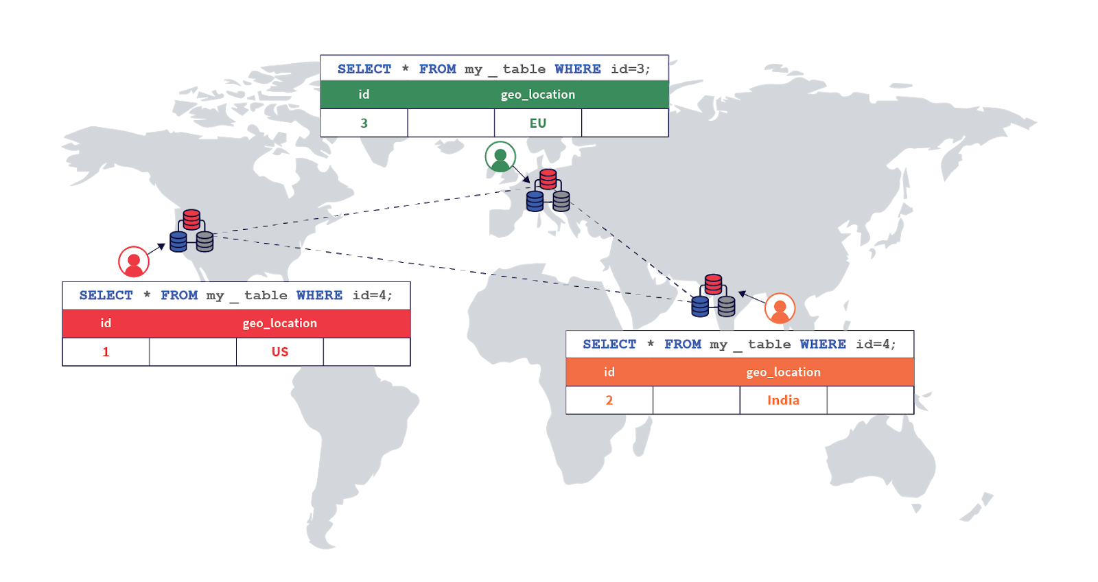
In this deployment, users can access their data with low latencies because the data resides on servers that are geographically close by, and the queries do not need to access data in far away geographic locations.

This tutorial explains this feature in the context of an example scenario described in the next section.

Example scenario

Let us look at this feature in the context of a use case. Say that a large but imaginary bank, Yuga Bank, wants to offer an online banking service to users in many countries by processing their deposits, withdrawals, and transfers.

The following attributes would be required in order to build such a service.

• Transactional semantics with high availability: Consistency of data is paramount in a banking application, hence the database should be ACID compliant. Additionally, users expect the service to always be available, making high availability and resilience to failures a critical requirement.
• High performance: The online transactions need to be processed with a low latency in order to ensure a good end-user experience. This requires that the data for a particular user is located in a nearby geographic region. Putting all the data in a single location in an RDBMS would mean the requests for users residing far away from that location would have very high latencies, leading to a poor user experience.
• Data residency requirements for compliance: Many countries have regulations around which geographic regions the personal data of their residents can be stored in, and bank transactions being personal data are subject to these requirements. For example, GDPR has a data residency stipulation which effectively requires that the personal data of individuals in the EU be stored in the EU. Similarly, India has a requirement issued by the Reserve Bank of India (or RBI for short) making it mandatory for all banks, intermediaries, and other third parties to store all information pertaining to payments data in India – though in case of international transactions, the data on the foreign leg of the transaction can be stored in foreign locations.

Step 1. Create table with partitions

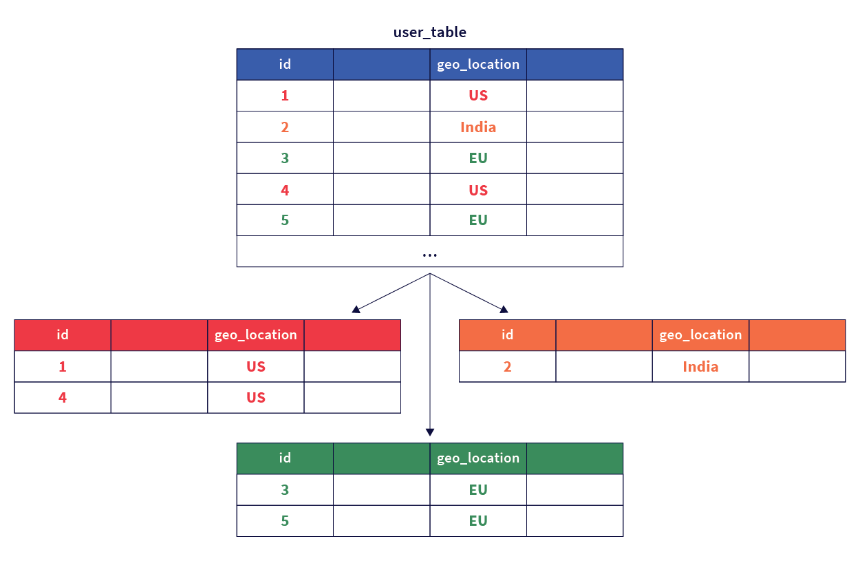
First, we create the parent table that contains a geo_partition column which is used to create list-based partitions for each geographic region we want to partition data into as shown in the following diagram:

1. Create the parent table.

   CREATE TABLE transactions (
       user_id   INTEGER NOT NULL,
       account_id INTEGER NOT NULL,
       geo_partition VARCHAR,
       account_type VARCHAR NOT NULL,
       amount NUMERIC NOT NULL,
       txn_type VARCHAR NOT NULL, 
       created_at TIMESTAMP DEFAULT NOW()
   ) PARTITION BY LIST (geo_partition);
   

2. Create tablespaces for each region.

   CREATE TABLESPACE eu_central_1_tablespace WITH (
     replica_placement='{"num_replicas": 3, "placement_blocks":
     [{"cloud":"aws","region":"eu-central-1","zone":"eu-central-1a","min_num_replicas":1},
     {"cloud":"aws","region":"eu-central-1","zone":"eu-central-1b","min_num_replicas":1},
     {"cloud":"aws","region":"eu-central-1","zone":"eu-central-1c","min_num_replicas":1}]}'
   );
   
   CREATE TABLESPACE us_west_2_tablespace WITH (
     replica_placement='{"num_replicas": 3, "placement_blocks":
     [{"cloud":"aws","region":"us-west-2","zone":"us-west-2a","min_num_replicas":1},
     {"cloud":"aws","region":"us-west-2","zone":"us-west-2b","min_num_replicas":1},
     {"cloud":"aws","region":"us-west-2","zone":"us-west-2c","min_num_replicas":1}]}'
   );
   
   CREATE TABLESPACE ap_south_1_tablespace WITH (
     replica_placement='{"num_replicas": 3, "placement_blocks":
     [{"cloud":"aws","region":"ap-south-1","zone":"ap-south-1a","min_num_replicas":1},
     {"cloud":"aws","region":"ap-south-1","zone":"ap-south-1b","min_num_replicas":1},
     {"cloud":"aws","region":"ap-south-1","zone":"ap-south-1c","min_num_replicas":1}]}'
   );
   

3. Next, create one partition per desired geography under the parent table, and assign each to the applicable tablespace. Here, you create three table partitions: one for the EU region called transactions_eu, another for the India region called transactions_india, and a third default partition for the rest of the regions called transactions_default.

   CREATE TABLE transactions_eu 
       PARTITION OF transactions 
         (user_id, account_id, geo_partition, account_type, 
         amount, txn_type, created_at,
         PRIMARY KEY (user_id HASH, account_id, geo_partition))
       FOR VALUES IN ('EU') TABLESPACE eu_central_1_tablespace;;
   
   CREATE TABLE transactions_india 
       PARTITION OF transactions
         (user_id, account_id, geo_partition, account_type, 
         amount, txn_type, created_at,
         PRIMARY KEY (user_id HASH, account_id, geo_partition))
       FOR VALUES IN ('India') TABLESPACE ap_south_1_tablespace;
   
   CREATE TABLE transactions_default 
       PARTITION OF transactions
         (user_id, account_id, geo_partition, account_type, 
         amount, txn_type, created_at,
         PRIMARY KEY (user_id HASH, account_id, geo_partition))
       DEFAULT TABLESPACE us_west_2_tablespace;
   

4. Use the \d command to view the table and partitions you've created so far.

   yugabyte=# \d
   

                   List of relations
    Schema |         Name         | Type  |  Owner
   --------+----------------------+-------+----------
   public | transactions         | table | yugabyte
   public | transactions_default | table | yugabyte
   public | transactions_eu      | table | yugabyte
   public | transactions_india   | table | yugabyte
   (4 rows)
   

The data is now arranged as follows:

Step 2. Pinning user transactions to geographic locations

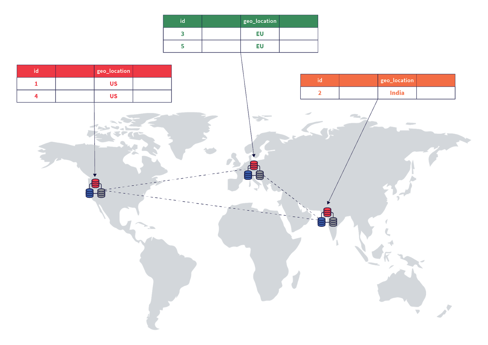
Now, the setup should automatically be able to pin rows to the appropriate regions based on the value set in the geo_partition column. This is shown in the following diagram:

You can test this region pinning by inserting a few rows of data and verifying they are written to the correct partitions.

yugabyte=# \x auto

Expanded display is used automatically.

1. Insert a row into the table with the geo_partition column value set to EU below.

   INSERT INTO transactions 
       VALUES (100, 10001, 'EU', 'checking', 120.50, 'debit');
   

2. Verify that the row is present in the transactions table.

   yugabyte=# select * from transactions;
   

   -[ RECORD 1 ]-+---------------------------
   user_id       | 100
   account_id    | 10001
   geo_partition | EU
   account_type  | checking
   amount        | 120.5
   txn_type      | debit
   created_at    | 2020-11-07 21:28:11.056236
   

Additionally, the row must be present only in the transactions_eu partition, which can be easily verified by running the select statement directly against that partition. The other partitions should contain no rows.

yugabyte=# select * from transactions_eu;

-[ RECORD 1 ]-+---------------------------
user_id       | 100
account_id    | 10001
geo_partition | EU
account_type  | checking
amount        | 120.5
txn_type      | debit
created_at    | 2020-11-07 21:28:11.056236

yugabyte=# select count(*) from transactions_india;

 count
-------
     0

yugabyte=# select count(*) from transactions_default;

 count
-------
     0

Now, let's insert data into the other partitions.

INSERT INTO transactions 
    VALUES (200, 20001, 'India', 'savings', 1000, 'credit');
INSERT INTO transactions 
    VALUES (300, 30001, 'US', 'checking', 105.25, 'debit');

These can be verified as follows:

yugabyte=# select * from transactions_india;

-[ RECORD 1 ]-+---------------------------
user_id       | 200
account_id    | 20001
geo_partition | India
account_type  | savings
amount        | 1000
txn_type      | credit
created_at    | 2020-11-07 21:45:26.011636

yugabyte=# select * from transactions_default;

-[ RECORD 1 ]-+---------------------------
user_id       | 300
account_id    | 30001
geo_partition | US
account_type  | checking
amount        | 105.25
txn_type      | debit
created_at    | 2020-11-07 21:45:26.067444

Step 4. Users travelling across geographic locations

In order to make things interesting, let us say user 100, whose first transaction was performed in the EU region travels to India and the US, and performs two other transactions. This can be simulated by using the following statements.

INSERT INTO transactions 
    VALUES (100, 10001, 'India', 'savings', 2000, 'credit');
INSERT INTO transactions 
    VALUES (100, 10001, 'US', 'checking', 105, 'debit');

Now, each of the transactions would be pinned to the appropriate geographic locations. This can be verified as follows.

yugabyte=# select * from transactions_india where user_id=100;

-[ RECORD 1 ]-+---------------------------
user_id       | 100
account_id    | 10001
geo_partition | India
account_type  | savings
amount        | 2000
txn_type      | credit
created_at    | 2020-11-07 21:56:26.760253

yugabyte=# select * from transactions_default where user_id=100;

-[ RECORD 1 ]-+---------------------------
user_id       | 100
account_id    | 10001
geo_partition | US
account_type  | checking
amount        | 105
txn_type      | debit
created_at    | 2020-11-07 21:56:26.794173

All the transactions made by the user can efficiently be retrieved using the following SQL statement.

yugabyte=# select * from transactions where user_id=100 order by created_at desc;

-[ RECORD 1 ]-+---------------------------
user_id       | 100
account_id    | 10001
geo_partition | US
account_type  | checking
amount        | 105
txn_type      | debit
created_at    | 2020-11-07 21:56:26.794173
-[ RECORD 2 ]-+---------------------------
user_id       | 100
account_id    | 10001
geo_partition | India
account_type  | savings
amount        | 2000
txn_type      | credit
created_at    | 2020-11-07 21:56:26.760253
-[ RECORD 3 ]-+---------------------------
user_id       | 100
account_id    | 10001
geo_partition | EU
account_type  | checking
amount        | 120.5
txn_type      | debit
created_at    | 2020-11-07 21:28:11.056236

Step 5. Adding a new geographic location

Assume that after a while, our fictitious Yuga Bank gets a lot of customers across the globe, and wants to offer the service to residents of Brazil, which also has data residency laws. Thanks to row-level geo-partitioning, this can be accomplished easily. We can simply add a new partition and pin it to the AWS South America (São Paulo) region sa-east-1 as shown below.

CREATE TABLESPACE sa_east_1_tablespace WITH (
    replica_placement='{"num_replicas": 3, "placement_blocks":
      [{"cloud":"aws","region":"sa-east-1","zone":"sa-east-1a","min_num_replicas":1},
      {"cloud":"aws","region":"sa-east-1","zone":"sa-east-1b","min_num_replicas":1},
      {"cloud":"aws","region":"sa-east-1","zone":"sa-east-1c","min_num_replicas":1}]}'
    );

CREATE TABLE transactions_brazil
    PARTITION OF transactions
      (user_id, account_id, geo_partition, account_type,
       amount, txn_type, created_at,
       PRIMARY KEY (user_id HASH, account_id, geo_partition))
    FOR VALUES IN ('Brazil') TABLESPACE sa_east_1_tablespace;

And with that, the new region is ready to store transactions of the residents of Brazil.

INSERT INTO transactions 
    VALUES (400, 40001, 'Brazil', 'savings', 1000, 'credit');

select * from transactions_brazil;

-[ RECORD 1 ]-+-------------------------
user_id       | 400
account_id    | 40001
geo_partition | Brazil
account_type  | savings
amount        | 1000
txn_type      | credit
created_at    | 2020-11-07 22:09:04.8537